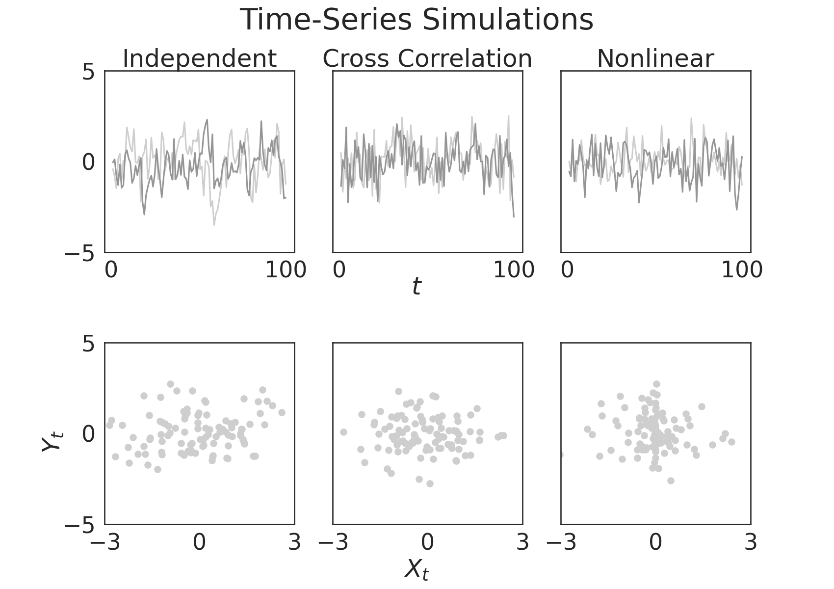
Time-Series Sims

Time-series simulations are found in hyppo.tools. Here, we visualize what these simulations look like.

import matplotlib.pyplot as plt
import seaborn as sns
from hyppo.tools import cross_corr_ar, indep_ar, nonlinear_process

# make plots look pretty
sns.set(color_codes=True, style="white", context="talk", font_scale=2)
PALETTE = sns.color_palette("Greys", n_colors=9)
sns.set_palette(PALETTE[2::2])

# constants
N = 100

# dictionary mapping of simulations
SIMULATIONS = [
    (indep_ar, "Independent"),
    (cross_corr_ar, "Cross Correlation"),
    (nonlinear_process, "Nonlinear"),
]


# make a function to plot the guassian simulations
def plot_time_series_sims():
    """Plot simulations"""
    fig, ax = plt.subplots(nrows=2, ncols=3, figsize=(17, 12))

    plt.suptitle("Time-Series Simulations", y=0.95, va="baseline")

    for i, row in enumerate(ax):
        for j, col in enumerate(row):
            sim, sim_title = SIMULATIONS[j]

            # time-series simulation
            x, y = sim(N)
            n = x.shape[0]
            t = range(1, n + 1)

            if i == 0:
                col.plot(t, x, label="X_t")
                col.plot(t, y, label="Y_t")

            else:
                col.scatter(x, y)

            # make the plot look pretty
            col.set_yticks([])
            if j == 0:
                col.set_yticks([-5, 0, 5])
            if i == 1:
                col.set_xticks([-3, 0, 3])
                col.set_xlim(-3, 3)
            if i == 0:
                col.set_title("{}".format(sim_title))
                col.set_xticks([0, 100])
            col.set_ylim(-5, 5)

    plt.subplots_adjust(hspace=0.5)
    fig.text(0.5, 0.02, r"$X_t$", ha="center")
    fig.text(0.5, 0.5, r"$t$", ha="center")
    fig.text(0.05, 0.25, r"$Y_t$", va="center", rotation="vertical")


# run the created function for the time-series simulations
plot_time_series_sims()

previous

K-Sample Sims

next

Independence Testing